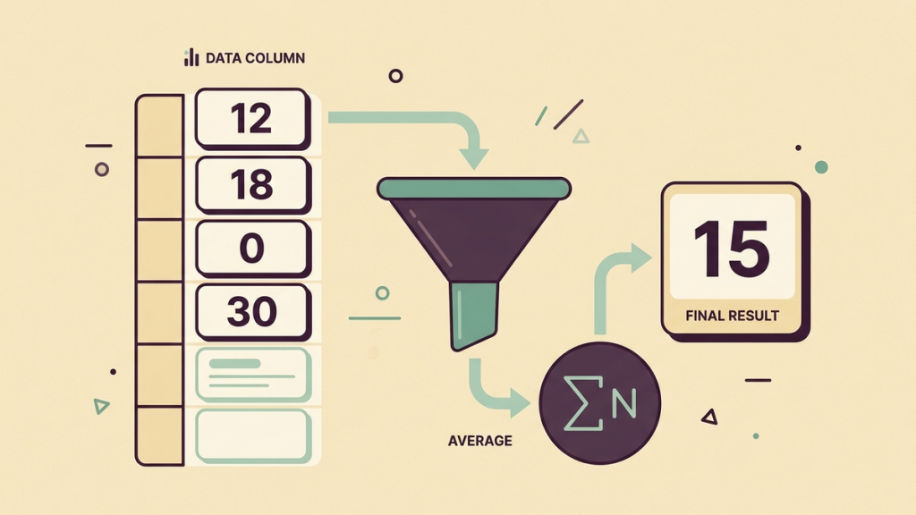
Enter =AVERAGE(B2:B7) to calculate the arithmetic mean of the numeric values in cells B2 through B7. Google Sheets adds the numbers and divides by the number of numeric observations.
If the answer looks wrong, the formula may be working correctly on data you did not intend to include. Blank cells, zeros, text, and unequal group sizes are the first things to investigate.
I used AVERAGE. Why did I get 15?
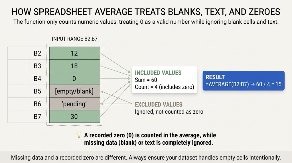
Consider this sheet of completed tasks:
|
Cell |
Entry |
Included in the mean? |
|---|---|---|
|
B2 |
12 |
Yes |
|
B3 |
18 |
Yes |
|
B4 |
0 |
Yes |
|
B5 |
Empty cell |
No |
|
B6 |
pending |
No |
|
B7 |
30 |
Yes |
The formula is:
=AVERAGE(B2:B7)
The four numeric entries total 60. Therefore, the average is 60/4 = 15. It is not 10, because the empty cell and the text “pending” are not two extra zero observations.
Google’s AVERAGE function reference confirms that the function averages numeric values and ignores text in the supplied range.
This makes the meaning of a missing entry important. A day with no completed tasks belongs in the sheet as zero. A day whose result has not been recorded is missing information. Treating the two as interchangeable changes what the average describes.
How do I average a whole column?
For a growing list with a text heading in B1, use:
=AVERAGE(B2:B)Place the formula somewhere outside that range, such as D2. Putting it in column B below the data while averaging B2:B can make it include itself and create a circular reference.
An open-ended range is convenient, but it also includes numeric notes or totals that someone may add farther down the column. For a fixed assignment or monthly report, a bounded range such as B2:B31 is easier to audit.
To average a row instead, change the range direction:
=AVERAGE(B2:F2)Select only the observations you intend to summarize. A total row is not an extra observation.
Can I ignore zeros?
Yes, but decide whether excluding them makes sense before changing the formula.
For the example range, use:
=AVERAGEIF(B2:B7,"<>0")This averages the nonzero numeric values 12, 18, and 30, giving 20. It answers “What was the average among observations that were not zero?” It does not answer the same question as the original mean of 15.
The AVERAGEIF documentation describes averaging values that satisfy a condition. The condition “<>0” means not equal to zero. It does not mean positive: negative values are also nonzero.
For instance, if zero means a shop made no sales that day, removing it makes the average daily sales look higher. Excluding zero is appropriate only when that exclusion matches the question you are trying to answer.
Why are some imported numbers being ignored?
A cell can look numeric while containing text. An apostrophe before a number, an unexpected decimal separator, or copied formatting can prevent the value from being treated as a number.
Test a suspicious cell:
=ISNUMBER(B2)TRUE means Sheets recognizes a number. FALSE tells you to inspect the value. To compare the numeric count with the number of filled cells in a range, use:
=COUNT(B2:B7)
=COUNTA(B2:B7)
These counts can differ because COUNTA also counts text and other nonempty entries. A difference is a clue, not proof that every extra entry is an error.
For a simple numeric string, =VALUE(B2) may convert it. Test the conversion on a copy, especially with commas, periods, dates, or currency symbols. Locale conventions matter: “1,500” can be interpreted differently from “1.500” in different settings.
Do not replace every unrecognized entry with zero. A note such as “not recorded” contains no measurement to average.
How do I average only one category?
Suppose A2:A20 contains department names and B2:B20 contains task counts. To average the numeric counts for Support, use:
=AVERAGEIF(A2:A20,"Support",B2:B20)The first range identifies the category. The final range supplies the numbers being averaged. Keep the ranges aligned so each category is matched with the correct observation.
This is different from filtering your view and assuming the ordinary AVERAGE formula now covers only visible rows. A filter changes what you see; it does not rewrite the range inside your formula. For visible-row calculations, use a suitable function and verify its filtering behavior separately.
Can I average the averages?
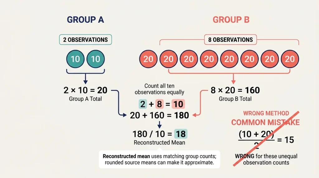
Not always. Suppose a small group has two observations averaging 10, while a larger group has eight observations averaging 20.
The simple average of 10 and 20 is 15. But the combined mean of all ten observations is:
(10 x 2 + 20 x 8) / (2 + 8) = 18
Put the group means in B2:B3 and the group counts in C2:C3. A weighted calculation is:
=SUMPRODUCT(B2:B3,C2:C3)/SUM(C2:C3)This assumes the counts are the appropriate nonnegative weights and their total is greater than zero. If group means were rounded before you received them, the reconstructed overall mean is also approximate. Original totals and counts are better when available.
Should I round the formula or just the display?
Use number formatting when you simply want a shorter-looking result. For example, showing two decimal places can display 15.3333… as 15.33 while retaining the underlying value for later calculations.
Use =ROUND(AVERAGE(B2:B7),2) only when the calculation itself should return a value rounded to two decimals. Rounding too early can change later totals or comparisons.
If a range contains no numeric values, an average has no valid denominator. Investigate empty or text-only input rather than reporting a made-up zero.
As a final check, manually calculate the average by adding all the values and dividing the total by the number of values. You can also use an online average calculator to double-check your result. Make sure you use the same values in both calculations, especially if your spreadsheet has filters applied.